using CairoMakie
using MetricSpaces
using MetricSpaces.Datasets
using TDAplots
using TDAmapper.ImageCovers
using TDAmapper.IntervalCovers
using TDAmapper.Refiners10 (Classical) mapper
10.1 Reeb graph
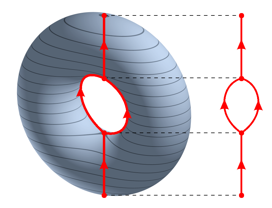
In topology, one way to visualize a complicated space is to collapse the connected components of the level sets of a function \(f : X \to \mathbb{R}\). The result is the Reeb graph.
So instead of trying to look directly at a high-dimensional object, we look at how it changes along the values of a function. The Reeb graph records how those level sets split, merge, and loop.
10.1.1 The classical Mapper construction
Mapper is the data-analytic analogue of the Reeb graph. We replace the continuous ingredients by discrete ones:
- \(X\) becomes a finite metric space, or point cloud;
- \(f : X \to \mathbb{R}\) becomes any real-valued function on the data;
- instead of inverse images of points, we use inverse images of overlapping intervals;
- instead of connected components, we cluster each inverse image.
The resulting clusters form a cover of the data, and the Mapper graph is the nerve of that cover: two nodes are connected when the corresponding clusters share at least one data point.
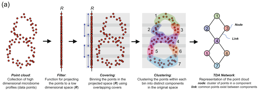
This graph can shed light on the geometry of the dataset:
- nodes represent clusters of data points;
- node colors summarize some statistic of the points in that node;
- edges indicate overlap between nearby clusters;
- loops suggest circular or toroidal structure;
- branches suggest flares or bifurcations in the data.
10.2 An example in Julia
We work with a torus. It is a useful example because its Reeb graph under a coordinate projection has a recognizable loop-with-flares structure:
X = torus(2000)
fv = first.(X)
Xmat = as_matrix(X)

fig = Figure()
ax = Axis3(fig[1, 1], title = "Torus colored by the filter value")
scatter!(ax, Xmat[1, :], Xmat[2, :], Xmat[3, :], color = fv, markersize = 3)
fig
The filter function is simply the projection onto the first coordinate:
fv[1:5]5-element Vector{Float64}:
-2.1088042762546406
2.3569091653320293
-3.2820301211629586
2.8847367015372667
-2.436282056039335To run classical Mapper we need:
- an image cover of the filter values;
- a clustering rule for each inverse image.
Here Uniform(length = 12, expansion = 0.35) creates overlapping intervals in the image of the filter, and DBscan refines each inverse image into connected dense pieces.
C = R1Cover(fv, Uniform(length = 12, expansion = 0.35))
clustering = DBscan(radius = 1.2, min_neighbors = 3)

mp = classical_mapper(X, C, clustering)
mp
Mapper graph with 16 vertices and 16 edgesAnd now we plot the Mapper graph, coloring each node by the mean filter value of the points it contains:
mapper_plot(mp, node_values = node_colors(mp, fv))
The graph has the same qualitative feature as the Reeb graph of a torus: a looped structure with two flaring sides. That is exactly what Mapper is supposed to do: replace a complicated point cloud by a graph that still reflects the large-scale shape.
10.3 A note on data representation
The local JuliaTDA packages work natively with EuclideanSpace objects from MetricSpaces.jl. If your data starts life as a d \times n matrix with one point per column, EuclideanSpace(M) converts it to the representation expected by TDAmapper.jl. When you want a matrix back for plotting, use as_matrix(X).
So the original column-major convention of the book is still there conceptually; it is just wrapped in a metric-space type that keeps the downstream API cleaner.
https://commons.wikimedia.org/wiki/File:3D-Leveltorus-Reebgraph.png↩︎