11 Ball mapper – Topological Data Analysis with Julia

11.1 The Vietoris-Rips complex

Another way to reduce the complexity of a metric space is to approximate it by a simplicial complex. Simplicial complexes are like small building blocks glued together: points, line segments, triangles, tetrahedra, and their higher-dimensional analogues.

The Vietoris-Rips complex is defined from a metric space \((X, d)\) and a scale \(\epsilon > 0\) by

\[ VR(X, \epsilon) = \{ [x_1, \ldots, x_n] \; ; \; d(x_i, x_j) < \epsilon \text{ for all } i,j \}. \]

So the vertices are the points of \(X\), and we add a simplex whenever all of its vertices are pairwise close enough. This is one of the most common ways to turn a metric space into a combinatorial object.

The black dots are points in a metric space; the pink circles are \(\epsilon\)-balls around the points; in green, we have the Vietoris-Rips complex. Source: https://www.researchgate.net/publication/331739415_Topological_data_analysis_for_the_string_landscape

11.2 The ball mapper

Ball Mapper is clearly inspired by the Vietoris-Rips complex, but it restricts the centers of the balls to a chosen subset of landmark points. Given a metric space \((X, d)\), a subset of indices \(L \subseteq \{1, \ldots, n\}\), and a radius \(\epsilon\), we place an \(\epsilon\)-ball around each landmark and connect two landmarks when their balls overlap.

In that sense, Ball Mapper can be viewed as a landmark-based simplification of the 1-skeleton of a Rips-like construction: it keeps the large-scale geometry while using far fewer centers than the full dataset.

11.3 Example in Julia

using CairoMakie
using MetricSpaces
using MetricSpaces.Datasets
using TDAplots
using Random

To exemplify, consider a circle:

X = sphere(1000, dim = 2)
metricspace_plot(X, markersize = 4)

Now choose 100 landmarks with farthest-point sampling and build the Ball Mapper graph:

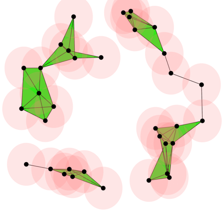
L = farthest_points_sample_ids(X, 100)
bm = ball_mapper(X, L, 0.35)

Mapper graph with 100 vertices and 1078 edges

mapper_plot(bm, node_values = node_colors(bm, first.(X)))

The resulting graph is a combinatorial shadow of the circle: it keeps the loop, but with far fewer nodes than the original point cloud. That is the point of Ball Mapper: summarize shape without carrying every point around.

11.4 Remarks

The landmark set \(L\) controls the resolution.
The radius \(\epsilon\) controls how much overlap we allow between neighboring balls.
If \(\epsilon\) is too small, the graph becomes disconnected.
If \(\epsilon\) is too large, the graph collapses and loses shape information.

Ball Mapper is especially useful when the raw point cloud is large, because it compresses the dataset before building the graph.